Does splitting vLLM Prefill/Decode across two B200s actually make things faster?
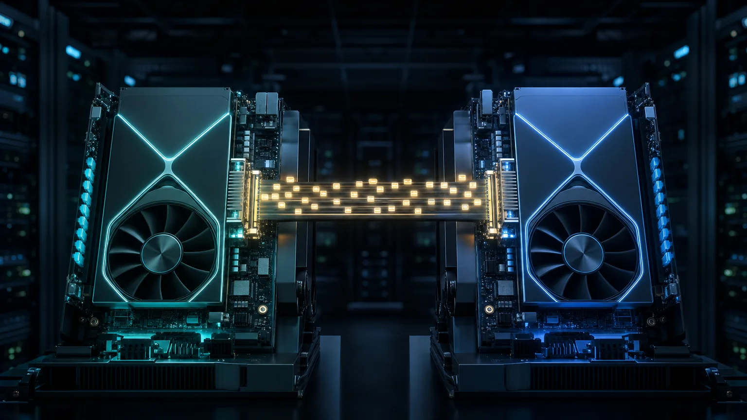 A depiction of a disaggregated serving setup where one GPU handles Prefill and the other handles Decode, with the KV cache crossing over NVLink.
Overview
“If you have two GPUs, wouldn’t it be faster to run Prefill and Decode separately?” is a thought that crosses the mind of anyone who works on serving. We verified that hypothesis on actual hardware. On two NVIDIA B200 GPUs, we ran three configurations with vLLM 0.24 against the same workload and measured tokens generated per second (TPS). The target models were two: Qwen3.6-27B-NVFP4, released by NVIDIA, and gemma-4-26B-A4B-it-FP8-Dynamic, released by RedHat.
To state the conclusion first, in an environment with only two GPUs, the winner for total throughput was not Prefill/Decode disaggregation. Disaggregation actually had the lowest total TPS, and instead delivered its value by lowering inter-token latency by three to four times on traffic with long inputs and short outputs. However, this result does not contradict the large performance gains reported by NVIDIA or by large-scale Chinese serving cases. The benefit of disaggregation is an optimization that depends on scale and SLOs, and we measured only the small end of that curve. So this post covers not only our measured numbers and the process of getting a bare-metal B200 running, but also a decision guide for when to disaggregate and when to just go with data parallelism or tensor parallelism, drawing on the evidence from DistServe, Splitwise, Mooncake, DeepSeek, and NVIDIA Dynamo.
Why we ran this experiment
Prefill and Decode are operations with different characters. Prefill is a compute-intensive stage that pushes the entire input through at once, while Decode is a memory-bandwidth-intensive stage that pulls out tokens one at a time. When the two are mixed on one GPU, a heavy Prefill cuts into the Decode stream, causing tokens to stutter. That is why, in large clusters, disaggregation, splitting into Prefill-only nodes and Decode-only nodes, is becoming the standard.
The problem arises when there are “exactly two GPUs.” If you tie up one GPU as Prefill-only, that GPU sits idle while Decode is busy, and it cannot help Decode even when Prefill is idle. So instead of assuming disaggregation is beneficial, we decided to set up data parallelism, which simply replicates the same model across both GPUs, as a formal competitor and let measurement decide.
Experiment environment
The host was bare metal with only the driver installed; the rest of the software stack was confirmed and finalized while running the experiments.
| Item | Value |
|---|---|
| GPU | NVIDIA B200 x 2 (183GB HBM each), NVLink (NV18) between GPU0 and GPU1 |
| Driver | 580.95.05 (CUDA 13 series) |
| vLLM / torch | vLLM 0.24.0 / torch 2.11.0+cu130 |
| Attention backend | Triton (FlashInfer JIT unavailable because the host lacked the CUDA toolkit’s nvcc) |
| Model A | nvidia/Qwen3.6-27B-NVFP4 (dense 27B, hybrid attention, NVFP4 weights + FP8 KV) |
| Model B | RedHatAI/gemma-4-26B-A4B-it-FP8-Dynamic (MoE 26.5B, 4B active, FP8 W8A8) |
Both models’ weights fit on a single B200. NVFP4 is about 15GB and FP8 is about 27GB, so there is no need to split them with tensor parallelism. So we compared three configurations that use both GPUs: TP=2, spreading one instance across both GPUs with tensor parallelism; DP=2, data parallelism placing two replicas on each GPU; and disaggregated 1P1D, placing Prefill on GPU0 and Decode on GPU1 and moving the KV cache over NIXL.
Measurement method
For load generation we used vLLM’s built-in vllm bench serve, and we set up the workload along two axes: one Decode-heavy traffic (input 512, output 2048), and one Prefill-heavy traffic (input 7500, output 200). Requests were all submitted at once to observe saturated throughput. The metrics we read were total output throughput (TPS) and inter-token latency (TPOT).
Server startup and benchmarking were run in the form below. The backend environment variables were required in this setup, and we explain why later.
# 공통 환경 (nvcc 부재 대응)
export VLLM_ATTENTION_BACKEND=TRITON_ATTN
export VLLM_USE_FLASHINFER_SAMPLER=0

# 데이터병렬 2복제 (한 엔드포인트, 두 장)
vllm serve $MODEL --data-parallel-size 2 --gpu-memory-utilization 0.90 \
  --max-model-len 32768 --trust-remote-code

# 벤치 (Decode 무거운 워크로드 예시)
vllm bench serve --model $MODEL --dataset-name random \
  --random-input-len 512 --random-output-len 2048 \
  --num-prompts 128 --request-rate inf --ignore-eos
For disaggregation, we started separate Prefill and Decode servers, attached the NixlConnector via --kv-transfer-config, and tied them together with the proxy vLLM provides.
# Prefill (GPU0, producer)
CUDA_VISIBLE_DEVICES=0 VLLM_NIXL_SIDE_CHANNEL_PORT=5600 \
vllm serve $MODEL --port 8100 --tensor-parallel-size 1 \
  --kv-transfer-config '{"kv_connector":"NixlConnector","kv_role":"kv_producer"}'

# Decode (GPU1, consumer)
CUDA_VISIBLE_DEVICES=1 VLLM_NIXL_SIDE_CHANNEL_PORT=5601 \
vllm serve $MODEL --port 8200 --tensor-parallel-size 1 \
  --kv-transfer-config '{"kv_connector":"NixlConnector","kv_role":"kv_consumer"}'
Results: Qwen3.6-27B-NVFP4
| Topology | Decode TPS | Prefill TPS | Decode TPOT | Prefill TPOT |
|---|---|---|---|---|
| DP=2 (Data Parallelism) | 8,245 | 2,230 | 11.4ms | 32.8ms |
| TP=2 (Tensor Parallelism) | 7,655 | 1,545 | 12.2ms | 44.1ms |
| 1P1D (Disaggregated) | 6,023 | 1,330 | 14.8ms | 9.9ms |
The picture is clear. Total TPS is highest for data parallelism on both workloads, and disaggregation comes last. On the Decode-heavy workload, data parallelism is 8% higher than tensor parallelism and 37% higher than disaggregation. On the Prefill-heavy workload the gap widens further, with data parallelism reaching 1.7 times disaggregation. With only two GPUs, tying up one GPU as Prefill-only means the idle time is charged back in full.
However, there is one column where disaggregation wins outright. The inter-token latency on the Prefill-heavy workload is 9.9ms, about a quarter of tensor parallelism’s 44ms or data parallelism’s 33ms. This is the reason disaggregation exists. In a mixed configuration, a heavy Prefill cuts into Decode and causes tokens to stutter, but in a disaggregated configuration the Decode-dedicated GPU is undisturbed by Prefill and tokens come out smoothly. The textbook explanation that disaggregation is a technique for evenness rather than volume shows up exactly in these numbers.
Results: gemma-4-26B-A4B-it-FP8-Dynamic
| Topology | Decode TPS | Prefill TPS | Decode TPOT | Prefill TPOT |
|---|---|---|---|---|
| TP=2 (Tensor Parallelism) | 7,069 | 1,730 | 13.6ms | 40.9ms |
| 1P1D (Disaggregated) | 5,766 | 1,474 | 17.9ms | 8.7ms |
| DP=2 (Data Parallelism) | Not measured | Not measured | Failed | Failed |
gemma is an MoE model, so its serving stack was trickier than the dense model’s. Tensor parallelism and disaggregation measured normally, but data parallelism failed to start on two separate attempts, both failing in the code path where vLLM 0.24 combines MoE with data parallelism. The first attempt died at a CUTLASS MoE warmup assertion, and the second attempt, with a lowered batched-token cap, died during the MoE forward pass of KV cache memory profiling. In other words, running gemma with data parallelism is currently not supported in this version, and that fact itself is a meaningful finding. MoE models have lower data parallelism stability than dense models. Comparing only the two configurations we could measure, the pattern that tensor parallelism beats disaggregation in total TPS holds for gemma as well. And disaggregation’s Prefill TPOT of 8.7ms overwhelming tensor parallelism’s 40.9ms is also the same as with Qwen.
So when do you disaggregate, and when do you just use DP/TP
A natural question arises here. NVIDIA’s blog and large-scale Chinese serving systems report large performance gains from disaggregation, so why is our result the opposite? Digging into the literature, the answer is clear. Our result does not contradict theirs. The benefit of disaggregation is an optimization that depends on scale and SLOs, not a universal win, and we simply measured the small end of that curve.
There is a paper that directly studies this crossover. “Beyond the Buzz: A Pragmatic Take on Inference Disaggregation” (arXiv:2506.05508) lays out that the benefit of disaggregation is greatest on Prefill-heavy traffic, while conversely, on Decode-centric traffic with long outputs, loose SLOs, or small models, piggybacking on the same GPU actually wins. It argues that for small models around 8B, the number of GPUs mapped to them is small, so there is little room to split Prefill and Decode in the first place, and the KV cache fits comfortably in HBM anyway, so there is no reason to move it. Our situation, running a 27B model on two GPUs, falls exactly in that range.
Conditions where disaggregation wins
Cases reporting large gains from disaggregation share common conditions. First, there are very many GPUs. UCSD Hao AI Lab’s retrospective describes the point where disaggregation becomes necessary as being in the hundreds-to-thousands-of-GPU range (retrospective post). Second, latency SLOs are tight. The core metric of DistServe (OSDI 2024), the flagship disaggregation paper, is not raw throughput but goodput, how many times more requests can be served while keeping SLOs above 90%. It reports withstanding much tighter SLOs on an A100 cluster tying together OPT 13B to 175B over NVLink (USENIX, arXiv:2401.09670). Third, large or MoE models are run with asymmetric parallelism. The DeepSeek-V3/R1 family reportedly split Prefill into narrow expert parallelism and Decode into wide expert parallelism, greatly raising Decode throughput compared to tensor parallelism, in a setup that spread Prefill across 4 nodes and Decode across 9 nodes on 96 H100 GPUs (LMSYS). Fourth, the KV cache is large and reused due to long context. Mooncake reports strength on long context through KV-cache-centric disaggregation (arXiv:2407.00079). Fifth, there is a high-speed fabric to move KV cheaply. Splitwise lowered transfer overhead by moving KV over InfiniBand, and Mooncake over hundreds-of-Gbps-class RDMA (Microsoft Research). The large multiples NVIDIA reports with Dynamo and GB200 NVL72 are also the result of running an ultra-large 671B-class model across racks at dozens-of-GPU scale (NVIDIA).
Conditions where DP/TP is better
Conversely, under the following conditions it is better to simply replicate with data parallelism or tensor parallelism. When the model is small enough to fit on one or two GPUs, when traffic is Decode-dominated because outputs are long, when the latency SLO is loose, when the GPUs are few enough that there isn’t enough headroom to keep separate Prefill and Decode pools from sitting idle, when it’s development or a low-QPS one-off workload where the complexity of disaggregated operations isn’t justified, and when inter-node bandwidth is PCIe-class rather than NVLink or InfiniBand class, so KV transfer itself becomes the bottleneck. Our 2xB200 experiment environment matches several items on this list exactly. The 27B model fits on one GPU, there are only two GPUs, and the goal was total throughput.
Four variables that decide the verdict
In the end, the choice is decided by a combination of four variables: the compute ratio between Prefill and Decode (the heavier Prefill is, the more disaggregation favors), the tightness of the latency SLO (the tighter, the more disaggregation favors), the scale of GPUs (the larger, the more disaggregation favors), and the savings from KV transfer relative to its cost (the larger and more reused the cache, or the faster the fabric, the more disaggregation favors). If even one of these points the other way, the benefit of disaggregation shrinks, and when a small number of GPUs, a small model, and a loose SLO all coincide, disaggregation is a net loss.
Summary of evidence
| System | Reported gain | Measured scale | Source |
|---|---|---|---|
| DistServe (OSDI’24) | 7.4x more requests or 12.6x tighter SLO while meeting SLOs | OPT 13B-175B, A100 NVLink cluster | arXiv:2401.09670 |
| Splitwise (ISCA’24) | 1.4x throughput (20% lower cost) or 2.35x throughput | Separate prompt/token pools, InfiniBand KV transfer | MS Research |
| Mooncake (Kimi) | Up to 525% throughput under simulated SLOs | Up to 800Gbps RDMA, long-context-centric | arXiv:2407.00079 |
| DeepSeek-V3/R1 | 5.2x Decode throughput vs TP | 96 H100 GPUs, Prefill 4 nodes / Decode 9-18 nodes | LMSYS |
| NVIDIA Dynamo + NVL72 | Up to tens of times on DeepSeek-R1 | 671B, GB200 NVL72 rack | NVIDIA |
| Beyond the Buzz (crossover study) | Gains shrink or reverse for small models, Decode-centric traffic, loose SLOs | Systematic study across models and scales | arXiv:2506.05508 |
In other words, disaggregation is a technique for the case of placing an ultra-large model across many GPUs and hitting a tight latency target over a high-speed fabric. If you are running a mid-sized model on two GPUs and targeting total throughput, data parallelism is the answer, and this is the conclusion that both our measurements and the literature point to together. The multiples above are values measured at the specific scale each paper studied, and some of them (Mooncake’s measured figures, TensorRT-LLM’s own numbers) are stated inconsistently across sources and should be re-checked before being quoted as-is.
Getting a bare-metal B200 running
As valuable as the numbers is the story of how we got it running. This host had only the driver installed and no inference stack, and we cleared the following walls one by one.
First, the CUDA compiler nvcc was missing, so FlashInfer failed when it tried to build its sampler and attention kernels at runtime. Switching the attention backend to Triton and turning off the FlashInfer sampler made things work normally. This also means that installing nvcc leaves room to push for higher TPS with FlashInfer’s Blackwell-native fast kernels.
Second, the first server startup took roughly 800 seconds, very long. This was due to torch.compile and CUDA graph capture, and with data parallelism, two engine cores compiling at the same time exceeded vLLM’s default readiness timeout of 600 seconds and died. We resolved this by raising the timeout to 1800 seconds.
Third, Qwen3.6’s hybrid attention has a Mamba-family conv state, and transferring it over NIXL required a specific conv state layout. Setting VLLM_SSM_CONV_STATE_LAYOUT=DS, as the error message indicated, made the KV transfer succeed, and a single accuracy check through the proxy verified that disaggregation was actually working correctly.
We recorded these findings as failure cases in a reusable experiment skill so we would not have to hit the same walls again. Making sure the next person doesn’t run into the same wall again is, we think, how you turn an experiment into an asset.
From ThakiCloud’s perspective
We build a sovereign AI platform that serves GPU inference on Kubernetes. The implication of this experiment for our operations is clear. Chasing trends with “disaggregation is the latest thing, so let’s disaggregate” can actually cut throughput in a small-GPU environment, while conversely, not using disaggregation in a large-scale, high-QPS service means missing latency SLOs. There is no single fixed answer, it is decided jointly by the four variables from the previous section: GPU scale and model size, the Prefill-to-Decode ratio of the traffic, the latency SLO, and fabric speed.
The problem is that this crossover differs from company to company and from workload to workload. Even the same 27B model, data parallelism is the answer on two GPUs, but if you place the same model across dozens of GPUs to serve long contexts under a tight SLO, disaggregation becomes the answer. Guessing at that boundary burns your GPU budget or misses your SLO. This is exactly the work we do. On our customers’ actual hardware and actual traffic, we pull per-topology numbers like in this post to find that boundary through measurement, and build a serving platform that switches between data parallelism, tensor parallelism, and disaggregation to match the workload. We also manage the benchmark pipeline and connection automation used in this experiment as reusable assets, so the same decision can be made in hours rather than days on the next model and the next hardware.
So if your team is adopting a new accelerator, whether B200 or H200, and needs to decide which topology fits your workload, we believe the fastest path is to work with us and settle that answer through measurement. Helping you decide with your own numbers instead of trends, that is the value ThakiCloud provides in inference optimization.
Conclusion and limitations
The measured answer to the question of serving these two models as fast as possible on 2xB200 is that if total throughput is the goal, it is data parallelism, not Prefill/Decode disaggregation. However, for a service where inputs are long, outputs are short, and the goal is low, even token latency, disaggregation lowers TPOT by three to four times, so in that case disaggregation is the answer. The choice is between throughput and latency stability, and this experiment attached real numbers to that trade-off.
We leave the limitations honestly on the table too. Because the attention backend was fixed to Triton, we did not measure the ceiling of Blackwell-native FlashInfer and the NVFP4 fast path. Installing nvcc is a follow-up task. We only looked at one saturation point of request rate and did not draw the full curve of latency versus throughput. Model-specific throughput levers such as Qwen’s multi-token-prediction speculative decoding and gemma’s expert parallelism are also left as follow-up axes. Adding these could raise the absolute numbers, but we expect the core conclusion of this experiment, that disaggregation across two GPUs is not for total throughput, will not change.
References
- Model A: nvidia/Qwen3.6-27B-NVFP4
- Model B: RedHatAI/gemma-4-26B-A4B-it-FP8-Dynamic
- vLLM distributed serving docs: docs.vllm.ai
- DistServe (OSDI 2024): arXiv:2401.09670
- Splitwise (ISCA 2024): Microsoft Research
- Mooncake (Kimi/Moonshot): arXiv:2407.00079
- DeepSeek large-scale expert parallelism: LMSYS blog
- NVIDIA Dynamo: NVIDIA developer blog
- Crossover study (Beyond the Buzz): arXiv:2506.05508
- 18-month disaggregated serving retrospective: Hao AI Lab